short title: Ipavich et al., The Solar Wind Proton Monitor
1Department of Physics, University of Maryland, College Park, Maryland
2Physikalisches Institut der Universität, Bern, Switzerland
3Institut für Datenverarbeitungsanlagen, Technische Universität, Braunschweig, Germany
4Max-Planck-Institut für extraterrestriche Physik, Garching, Germany
5Max-Planck-Institut für Aeronomie, Katlenburg-Lindau, Germany
6Department of Physics, University of Arizona, Tucson
7EOS, University of New Hampshire, Durham
8Institute for Space Physics, Moscow, Russia
9Jet Propulsion Laboratory, Pasadena
published in the Journal of Geophysical Research, 103, 17205, 1998
The Proton Monitor, a small subsensor in the CELIAS/MTOF experiment on the SoHO spacecraft, was designed to assist in the interpretation of measurements from the high mass resolution main MTOF sensor. In this paper we demonstrate that the Proton Monitor data may be used to generate reasonably accurate values of the solar wind proton bulk speed, density, thermal speed, and north/south flow direction. Correlation coefficients based on comparison with the solar wind measurements from the SWE instrument on the WIND spacecraft range from 0.87 to 0.99. Based on the initial 12 months of observations, we find that the proton momentum flux is almost invariant with respect to the bulk speed, confirming a previously published result. We present observations of two interplanetary shock events, and of an unusual solar wind density depletion. This large density depletion, and the correspondingly large drop in the solar wind ram pressure, may have been the cause of a nearly simultaneous large increase in the flux of relativistic magnetospheric electrons observed at geosynchronous altitudes by the GOES 9 spacecraft. Extending our data set with a 10-year time span from the OMNIWeb data set, we find an average frequency of about one large density depletion per year. The origin of these events is unclear; of the 10 events identified, 3 appear to be corotating and at least 2 are probably CME-related. The rapidly available, comprehensive data coverage from SoHO allows the production of near real time solar wind parameters that are now accessible on the World Wide Web.
The Solar and Heliospheric Observatory (SoHO) mission is a joint venture of the European Space Agency and the United States National Aeronautical and Space Administration. The SoHO spacecraft was launched on 2 December 1995, and was inserted into a halo orbit about the L1 Sun-Earth Lagrangian point in February 1996. The scientific payload may be broadly classified into three main research areas: helioseismology, upper solar atmosphere remote sensing, and solar particle in situ measurements [Domingo, Fleck and Poland, 1995]. One of the solar particle experiments is the Charge, Element, and Isotope Analysis System, CELIAS [Hovestadt et al., 1995]. The CELIAS package includes two sensors devoted to solar wind composition studies (Charge Time-of-Flight, CTOF, and Mass Time-of-Flight, MTOF) and one sensor devoted to solar wind proton measurements (the Proton Monitor, PM). Because of its position at L1, far upstream of the Earth's magnetosphere and the Earth's foreshock region, the SoHO spacecraft samples solar wind that has not been modified by the presence of the Earth. The spacecraft is three-axis stabilized, always facing the Sun. Hence the SoHO mission provides a ideal platform with excellent collection power for nearly continuous, undisturbed solar wind studies. In addition, the typical solar wind at the SoHO L1 location, about 1.5 million kilometers Sunward of the Earth, is observed nearly one hour before it reaches the Earth, thus allowing an early warning of possible impending magnetospheric disturbances.
The Proton Monitor (PM) is a subsensor of the MTOF experiment. MTOF determines high resolution mass spectra of heavy solar wind ions and uses a very wide bandwidth energy-per-charge analyzer to maximize counting statistics (at the expense of charge state information) for rare elements and isotopes. Since SOHO is not a spinning spacecraft, the deflection system was designed to have a wide angular acceptance in 2 dimensions. The PM was designed to assist in the interpretation of MTOF data and for that reason uses a similar wide bandwidth (and wide angular acceptance) analyzer that limits the accuracy of derived solar wind parameters. The original SoHO strawman payload included a traditional solar wind plasma experiment and magnetometer that were not able to be accommodated in the final instrument payload selection [Ness and Smith, 1988; Kivelson and Russell, 1988]. Consequently the Proton Monitor became the only SoHO sensor capable of determining the in situ solar wind proton speed, density or temperature. In order to partially recoup additional solar wind plasma information, an enhancement allowing the measurement of solar wind flow direction (in the plane out of the ecliptic) was subsequently approved by the project and added to the Proton Monitor design. The solar wind speed derived from the Proton Monitor is contributed to the International Solar Terrestrial Physics (ISTP) Program's "key parameters" database.
The Proton Monitor has the following science objectives:
In this paper we present a description of the SoHO Proton Monitor sensor, our analysis techniques, and some initial flight observations.
The Mass Time-Of-Flight (MTOF) experiment of the CELIAS investigation [Hovestadt et al., 1995] contains two sensors. The MTOF/Main is the primary unit, providing solar wind elemental and isotopic abundance measurements. The MTOF/Proton Monitor (PM) is a small auxiliary unit designed to measure the solar wind proton parameters, including speed and direction. Both units are housed within a common structure (see Figure 1), which also contains the low voltage power converter, the high voltage power supplies, the analog electronics, and the digital electronics. The smaller, leftmost, wedge-shaped black aperture in Figure 1 is the entrance to the Proton Monitor. (The larger wedge-shaped region is the opening to the Main sensor).
The MTOF Proton Monitor is a new type of solar wind Energy per Charge (E/Q) analyzer designed and fabricated by the University of Maryland. It consists of an electrostatic E/Q analyzer similar in form and function to the deflection system used in the MTOF/Main, and a MicroChannel Plate (MCP) detector with a two dimensional position sensing anode. The PM accepts ions from 0.3 to 6 keV/e with a minimum 2-dimensional angular acceptance of ±15° and a geometry factor of 1 x 10⁻⁴ cm2. The large angular acceptance is required since the SoHO spacecraft is 3-axis stabilized.
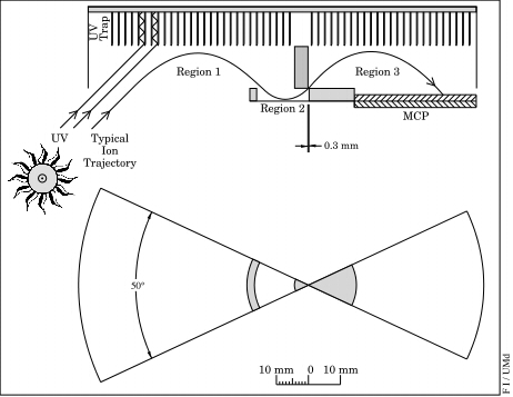
As illustrated in Figure 2, the E/Q analyzer consists of three 50° wedge-shaped parallel plate deflection regions. Each region is framed by Mecor walls with three linearly spaced thin gold-plated field control electrodes embedded in them. The front of each region through which particles pass is defined by a grid etched in a thin sheet of gold-plated Be-Cu. The back of regions 1 and 3 is open to a simple integrated aluminum UV-trap. Voltage is applied in four linear increments from 0 V on the grid to the appropriate positive voltages on the field control electrodes, and the highest voltage (* 4 kV) at the back of each region. The UV trap consists of a series of parallel thin (0.12 mm) flat metal fins (separated by 2 mm with a depth of 10 mm) oriented at an angle of 45 degrees to the nominal Sun-spacecraft line. The fins at the back of region 1 are coated with black Ni-Cr. This coating was chosen because of its light absorption properties, excellent electrical conductivity, and relative lack of contamination potential. Incoming photons that are specularly reflected must make at least 4 bounces before reaching the back of the UV trap. Several more bounces are required before the photon could enter region 2, which has a black Ni-Cr coating on its ceiling, and finally region 3 (which also has the aluminum fins, but no coating due to the proximity of the MCP). The three regions are cylindrically symmetric about a 0.3 mm diameter hole in the Be-Cu sheet between region 2 and region 3 (see Figure 2). The in-flight performance of the PM UV-trapping technique has been excellent. There is no measurable count rate attributable to UV, and after 20 months of exposure there is no evidence of degradation of the coatings.
Figure 3 (top) shows the entrance to region 1 (left), the back of region 2 (middle), and the back of the MCP (right). In Figure 3 (bottom) the MCP has been removed, exposing the exit grid for region 3 and the uncoated aluminum fins at the back of region 3. The MCP detector used in the PM is a custom wedge-shaped Chevronô design manufactured by Galileo Electro-Optics Corp. The Mecor MCP stack hardware separates the 2 plates (each 1 mm thick with 40:1 length/diameter ratio) by 0.25 mm. The front of the input plate is negatively biased and the anode is held at ground. In flight, the bias voltage across each plate is 950 v, the voltage across the gap separating the 2 plates is +40 v, and the anode is at +70 v with respect to the back of the output plate.
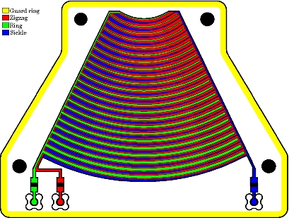
Figure 4 shows the cylindrically symmetric two-dimensional (R, q) position sensing anode, located 1 cm behind the output of the MCP. The anode uses a "sickle/ring" pattern [Knibbeler et al., 1987], with gold-plated copper elements etched on a ceramic substrate. Sickle-shaped elements with width varying linearly with angle provide angular position information. Radial position information is obtained from ring-shaped elements that change width linearly with radial distance from the apex of the anode pattern. A normalization element fills the gaps between the sickle and ring elements. Pulse height information from the three elements is used to calculate the radius and angle position using the following equations: R = Ring / (Ring + Sickle + Norm), q = Sickle / (Ring + Sickle + Norm). The energy-per-charge (and hence speed) of the incident ions is determined from the R (radial) position information, while the q position signal allows the determination of the solar wind flow angle in the plane perpendicular to the ecliptic plane.
The MTOF/PM data accumulation is organized within a commandable six-step deflection plate voltage sequence (5 seconds per step), thereby acquiring an entire E/Q spectrum every 30 seconds.
Our routine analysis to date has not included the Radius-position information that is available within each voltage step. This information, under conditions of low kinetic temperature, allows the derivation of the density of He++ in the solar wind. The q position information is being used to determine the solar wind H+ flow direction. The H+ bulk speed, thermal speed and density are derived from the sets of 6 rates (one for each voltage step of the PM deflection system) that are obtained every 30 seconds. In the nominal stepping sequence, the voltage steps are spaced logarithmically (60% step size) from 0.3 to 3 kV. At a given voltage step the energy per charge dynamic range is slightly more than a factor of 2. Two independent methods were used to derive the solar wind parameters: a fitting technique and a moment-calculating technique.
In the fitting method, solar wind parameters are derived by comparing the 6 measured rates with those resulting from a simulation program. The simulation assumes that solar wind protons may be represented by a convected Maxwellian distribution, characterized by a bulk speed and temperature. An alpha particle fraction of 4% is assumed. A heavy ion component with density of 0.025 of the He++ density is assumed at a mass/charge value of 2.7. The alphas and heavy ions are assumed to have the same temperature per mass as the protons. A fixed solar wind proton density (10 cm-3) is used in an analytic integration of the convected maxwellians over the bandwidth of the deflection system to derive the expected absolute counting rates.
The simulation assumes the following values of the 2 variables: The solar wind speed is allowed to vary from 235 km/s to 1042 km/s in 250 logarithmic steps of 0.6%; the Mach number (= ratio of bulk speed to the most probable thermal speed) is varied from 3.5 to 34.5 in 25 logarithmic steps of 10%. For each combination of the 2 variables a set of 6 rates is derived from the simulation. A total of 250 x 25 = 6250 'sextuplets' is thereby created. Each of the sextuplets is then compared with a measured set of 6 rates. For each comparison the sum of the 6 simulated rates is normalized to equal the sum of the 6 measured rates; the normalization factor is then used to derive the solar wind density. Finally, a goodness of fit parameter is used to select the best set of simulation parameters for a given set of 6 measured rates.
The second method uses simple numerical integration to calculate the moments of the distribution represented by the six rates. The density is derived from the weighted sum, the speed from the first moment, and the thermal speed from the square root of the second moment.
The q position signal (described in the Instrumentation section) is used by the Data Processing Unit to construct a set of 20 theta bins. The number of counts in each of these 20 angle bins (summed across all 6 voltage steps) are used to calculate an average bin number, from which the out-of-ecliptic angle is derived.
We have compared the PM solar wind parameters derived from both approaches with those derived from the SWE instrument on the WIND spacecraft (courtesy K. W. Ogilvie and A. J. Lazarus). The time period analyzed was 20 Jan 1996 to 31 Jan 1997. The SWE data consisted of Key Parameter data files (92 sec averages). Time periods when WIND had an XGSE position of < 50 Earth radii were deleted (to minimize the influence of the Earth's bow shock).
In order to partially compensate for the solar wind travel time between SoHO and WIND, the SWE data was shifted by a (constant) time, calculated as follows: The difference between the median XGSE coordinates for WIND and SoHO (116 and 220 RE, respectively) was divided by the average observed solar wind speed (420 km/s), yielding a median time delay of 26 min. Five-minute PM parameters were averaged over fixed 2-hour intervals. The SWE parameters, after time-shifting, were then averaged over the same 2-hour intervals. It was required that both instruments have at least 80% data coverage for a 2-hour interval to be accepted. Of the 4527 possible intervals, 4399 were accepted for SoHO and 3583 for Wind. The combined data set consisted of 3479 simultaneous 2-hour data points.
The SWE data set was used to refine the PM solar wind parameters derived from both the fitting and moment techniques. It was found that the moment technique produced higher correlation coefficients when compared to SWE parameters for bulk speed and thermal speed, while the fitting technique produced a higher correlation coefficient for density. The two techniques were then combined as follows. For the bulk speed, the ratio of PM (moment) and SWE values was correlated with the ratio of bulk speeds derived from the two techniques, and a correction function thereby obtained; the same was done for the thermal speed. For the density, the ratio of PM (fit technique) and SWE values was correlated with the density ratio derived from the two techniques to derive the correction function. Unless otherwise indicated, all results from the PM quoted below were obtained using this combined technique.
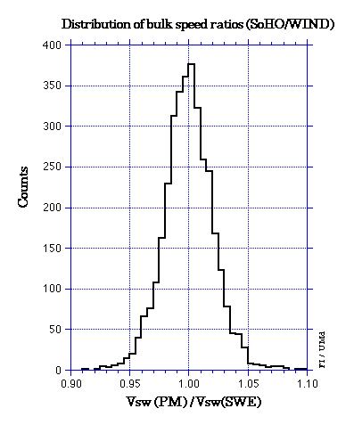
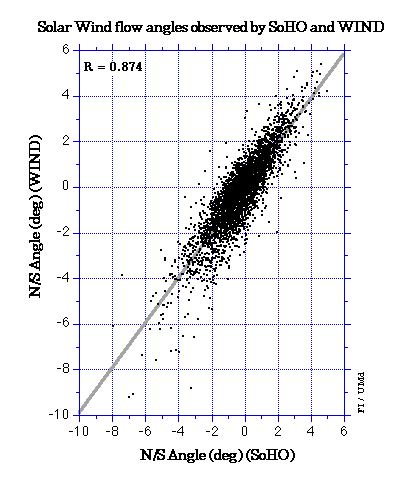
Figure 5 displays the frequency distribution of the ratio of the proton bulk speeds observed by PM and SWE. The standard deviations of the distribution of the ratios of solar wind parameters derived by the PM and SWE instruments are: 2.1% for the bulk speeds; 17% for the densities; and 16% for the thermal speeds. Some of the spread in these distributions is undoubtedly real, reflecting different solar wind conditions at the locations of the 2 spacecraft that are sometimes separated by more than 100 Earth radii in the YGSE direction. The correlation coefficients for the solar wind parameters from the two spacecraft are given in Table 1. A scatterplot of the solar wind flow angle (in the plane perpendicular to the ecliptic) observed simultaneously by the PM and SWE instruments is presented in Figure 6.
In this section we present a variety of inflight results obtained from the Proton Monitor.
Table 2 lists the average values of a number of standard solar wind proton parameters obtained from the data set discussed above (i.e., 2-hour averages, approximately 1 year data coverage). The standard deviation of the distribution is also listed for each parameter. It should be noted that the time period of these observations is basically during solar minimum conditions.
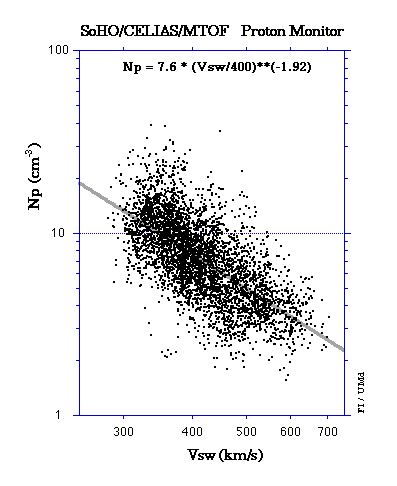
Figure 7 is a scatterplot of the solar wind proton density and bulk speed, obtained over the same ~ 1-year time period. A least squares power law fit to this data set has a slope of approximately -1.9; i.e., Np α Vsw-1.9. Hence the number flux (= Np· Vsw) varies as Vsw-0.9, and the momentum flux (= Np· mp· Vsw2, where mp is the proton mass) is nearly independent of speed, varying as Vsw+0.1. The kinetic energy flux (= 0.5 Np· mp· Vsw3) increases with speed, varying as Vsw+1.1.
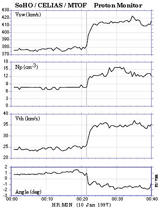
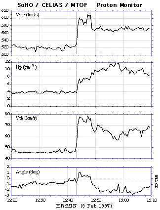
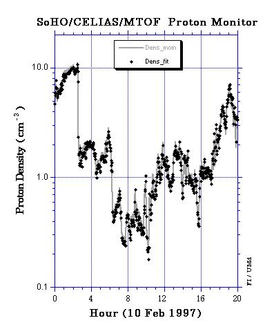
Figures 8 and 9 present PM measurements of probable interplanetary shock waves observed in early 1997, using the highest available time resolution (30 sec). Preliminary evidence from other SoHO experiments suggests that both of these shocks may be associated with CMEs (Coronal Mass Ejections). About 18 hours after the 9 Feb 1997 shock passage, the PM observed an unusual density depletion. Figure 10 presents the PM density measurements derived separately using the fitting and moment techniques discussed in the Analysis Section. The two techniques are in good agreement during this time period. The density remained below 1 cm-3 for about 5 hours, attaining a minimum value of about 0.2 cm-3. These are the lowest densities observed by the PM in its 20 months of operation. The solar wind speed during this period varied from about 420 to 470 km/s. Since SoHO has no magnetometer, we have used magnetic field data from the MFI instrument (courtesy R. P. Lepping) on the WIND spacecraft to estimate the local Alfven speed. At this time the GSE separation of the 2 spacecraft was about 1, 74 and 27 Earth radii in X, Y and Z, respectively. The magnetic field magnitude during the 5 hours of interest was quite steady with an average value of 8.5 nT. The peak calculated Alfven speed was about 420 km/s, somewhat less than the solar wind speed of 460 km/s at that time. The solar wind Alfven Mach number was thus quite low (about 1.1), but the solar wind was still super-Alfvenic.
The very low solar wind ram pressure at this time would be expected to cause the Earth's magnetopause and bow shock to expand much beyond their nominal locations. A possible consequence of this magnetospheric expansion is presented in Figure 11, which displays the flux of electrons with energies above 2 MeV observed by the geosynchronous GOES 9 spacecraft during 9-10 February 1997. The shaded region represents the time period (shifted by 1 hour to account for the solar wind propagation time from SoHO to the Earth) when the observed PM density was below 1 cm-3. A large increase in the electron flux appears to be initiated by the very low solar wind density. The peak flux attained on 10 February is unusually high; we have searched the previous 12 months of GOES data and found this to be the highest flux observed.
We have demonstrated that the Proton Monitor generates reasonably accurate solar wind proton parameters (see Table 1). The PM can identify interplanetary shocks (Figs 8 and 9) as well as very low density regions (Fig 10). Using the existing one-year PM database we have found that the solar wind proton momentum flux is very nearly independent of speed. The near invariance of the momentum flux has been emphasized by Schwenn [1990] based on analysis of Helios solar wind data from December 1974 to December 1976 (a period of low solar activity, as is the data set reported in this paper). Their average observed momentum flux (extrapolated from the Helios position to 1 AU) was 2.15 x 10⁻⁸ dynes/cm2 (equivalently, 2.15 nPa), essentially the same as our observed value (2.2 x 10⁻⁸ dynes/cm2, see Table 2). Phillips et al. [1996] presented an analysis of Ulysses solar wind proton data from September 1994 to June 1995, during which time the spacecraft traversed heliographic latitudes from -80.2 to +64.9. They found that the proton mass flux (equivalently proton number flux), scaled to 1 AU, was nearly constant with latitude, while the momentum flux was highest at high latitudes. This variable momentum flux (which is effectively the dynamic pressure exerted by the solar wind) led Phillips et al. [1996] to suggest a latitudinal asymmetry in the heliopause cross section. Since the solar wind speed is highly correlated with latitude, it is likely that for their data set the momentum flux also varies with speed, in contrast to the in-ecliptic results presented by Schwenn [1990] and in this work.
The very low solar wind density time period observed by SoHO (Fig 10) appears to be associated with a large increase in the flux of magnetospheric electrons with energies above 2 MeV observed by GOES 9 at geosynchronous altitudes (Fig 11). This flux increase (the largest in at least a year) may possibly have been caused by a non-adiabatic re-distribution of inner radiation belt electrons as the magnetosphere expanded in response to the very low solar wind ram pressure. Somewhat ironically, it may be that the strongest doses of relativistic electrons at geosynchronous altitudes may be the result of the very weakest solar wind.
One may ask how often the solar wind contains such very large density depletions. Recently Riley et al. [1997] reported a unique 'density hole' in their Ulysses spacecraft data set. The event, lasting about 3.5 hours, was observed at 3.7 AU and 38.5 heliographic latitude in the otherwise uniform fast solar wind. Gosling et al. [1982] presented ISEE 3 observations of several large density depletions. During portions of an ~ 5-hour long event on 22 November 1979 these authors report that the solar wind was sub-Alfvenic. The event was not associated with a shock or with a rarefaction region that could be dynamically produced in a region of declining solar wind speed. Gosling et al. [1982] also report a pair of density depletion events (July 4 and 31, 1979) that may have been caused by a quasi-stationary corotating structure.
In order to explore the systematics of large density depletions we have examined the NSSDC OMNIWeb data base, consisting of 1-hour averages of solar wind parameters. We considered the period from 1 January 1974 to 1 Jan 1984 (after this time the OMNIWeb data set may have artificially suppressed very-low densities [A. J. Lazarus, private communication, 1997]). The average data coverage was about 70% during this 10-year interval. Large density depletions were identified with those hourly intervals with an average proton density less than or equal to 0.5 cm-3. A total of 72 hourly intervals were found (out of a total of about 60,000 hours of data coverage). We further defined 'events' as contiguous or nearly contiguous groupings of these 72 intervals (intervals separated by less than 30 hours were considered part of the same event). This definition resulted in 9 events over the 10 year period. The average event duration, 8 hours, corresponds to a spatial scale of about 0.1 AU. The shortest event consisted of a single hourly average (6 June 1979) and the longest consisted of 20 hourly averages (31 July - 1 August 1979). Of the 9 events, 4 occurred in 1979. The 3 events reported by Gosling et al. [1982] were all identified with this analysis technique. In addition to the pair of density depletion events (July 4 and 31, 1979) identified by Gosling et al. [1982] as possibly being corotating, the OMNIWeb analysis identified an event on 6 June 1979 that is consistent with a third rotation; however, none of the other 9 events were corotating. The start of one of the events (1800 UT on 29 September 1978) occurred about 16 hours after the passage of a CME-associated interplanetary shock (the shock and CME were discussed by Ipavich et al., [1986] and Galvin et al., [1987]). The event on 10 February 1997 reported in the present work began about 18 hours after a CME-associated shock. Using the above event definition, the SoHO/PM data set produces one event in 20 months of data coverage; combined with the OMNIWeb analysis this results in an average frequency of about one large density depletion per year in the solar wind observed near Earth. The origin of these events remains unknown; of 10 total events, 3 appear to be corotating, and at least 2 are probably CME-related.
The excellent and rapid data availability from SoHO has allowed us to construct a page on the World Wide Web that presents Proton Monitor results on a near real time basis. The data are obtained by automatic electronic transfer from the Experimenters' Operations Facility at Goddard Space Flight Center to the University of Maryland. When files are received (typically every 30 minutes), several automated batch processes analyze and plot the data and dynamically update the Web page. The data on the Web page are typically between a few minutes and a few hours old. In addition to the most recent data, a catalog of 27-day (Carrington Rotation) plots are available from the Web page. The Proton Monitor data set is currently available on the World Wide Web at the following URL: https://space.umd.edu/pm.
Acknowledgments. We are very grateful to K. W. Ogilvie and A. J. Lazarus for the use of the WIND/SWE solar wind data set. We also thank R. P. Lepping for WIND/MFI magnetic field data, and acknowledge the use of the OMNIWeb database from the NSSDC, and the GOES data set from the U.S. Dept. of Commerce, NOAA, Space Environment Center. Finally, we thank the many individuals at the University of Maryland and the other CELIAS Institutions who contributed to the success of this experiment. This research was supported by NASA Grant NAG5-2754, the Swiss National Science Foundation, and by DARA, Germany under contracts 50 OC 89056 and 50 OC 96059.
W.I. Axford, H. Grünwaldt, M. Hilchenbach,
E. Marsch and B. Wilken, Max-Planck-Institut für Aeronomie, D-37189 Katlenburg-Lindau,
Germany. (e-mail: gruenwaldt@linax1.dnet.gwdg.de)
H. Balsiger, P. Bochsler, J. Geiss, S.
Hefti, R. Kallenbach and P. Wurz, Physikalisches Institut der Universität, CH-3012
Bern, Switzerland. (e-mail: bochsler@soho.unibe.ch)
A. Bürgi, D. Hovestadt, B. Klecker
and M. Scholer, Max-Planck-Institut für extraterrestriche Physik, D-85470 Garching,
Germany. (e-mail: bek@mpens.mpe-garching.mpg.de)
M.A. Coplan, A.B. Galvin, G. Gloeckler,
F.M. Ipavich, S.E. Lasley and J.A. Paquette, Department of Physics, University of
Maryland, College Park, MD 20742, USA. (e-mail: ipavich@umtof.umd.edu)
F. Gliem and K.-U. Reiche, Institut für
Datenverarbeitungsanlagen, Technische Universität, D-38023 Braunschweig, Germany.
(e-mail: gliem@ida.ing.tu-bs.de)
K.C. Hsieh, Department of Physics, University
of Arizona, Tucson, AZ 85721, USA. (e-mail: hsieh@soliton.physics.arizona.edu)
M.A. Lee and E. Möbius, EOS, University
of New Hampshire, Durham, NH 03824, USA. (e-mail: moebius@rotor.sr.unh.edu)
G.G. Managadze and M.I. Verigin, Institute
for Space Physics, Moscow, Russia. (e-mail: gmanagad@esoc.bitnet)
M. Neugebauer, Jet Propulsion Laboratory,
Pasadena, CA 91103, USA. (e-mail: mneugeb@jplsp.jpl.nasa.gov)
Domingo, V., B. Fleck, and A.I. Poland, The SOHO mission: an overview, Solar Physics 162, 1, 1995.
Galvin, A.B., F.M. Ipavich, G. Gloeckler, D. Hovestadt, S.J. Bame, B. Klecker, M. Scholer and B.T. Tsurutani, Solar wind iron charge states preceding a driver plasma, J. Geophys. Res., 92, 12069, 1987.
Hovestadt, D., M. Hilchenbach, A. Bürgi, B. Klecker, P. Laeverenz, M. Scholer, H. Grünwaldt, W.I. Axford, S. Livi, E. Marsch, B. Wilken, H.P. Winterhoff, F.M. Ipavich, P. Bedini, M.A. Coplan, A.B. Galvin, G. Gloeckler, P. Bochsler, H. Balsiger, J. Fischer, J. Geiss, R. Kallenbach, P. Wurz, K.-U. Reiche, F. Gliem, D.L. Judge, H.S. Ogawa, K.C. Hsieh, E. Mobius, M.A. Lee, G.G. Managadze, M.I. Verigin, and M. Neugebauer, CELIAS - charge, element, and isotope analysis system for SOHO, Solar Physics, 162, 441, 1995.
Gosling, J. T., J. R. Asbridge, S. J. Bame, W. C. Feldman, R. D. Zwickl, G. Paschmann, N. Sckopke, and C. T. Russell, A sub-Alfvenic solar wind: Interplanetary and magnetosheath observations, J. Geophys. Res., 87, 239, 1982.
Ipavich, F.M., A.B. Galvin, G. Gloeckler, D. Hovestadt, S.J. Bame, B. Klecker, M. Scholer, L.A. Fisk and C.Y. Fan, Solar wind Fe and CNO measurements in high speed flows, J. Geophys. Res., 91, 4133, 1986.
Kivelson, M.G., and C.T. Russell, Forum: SOHO: an unfortunate omission, Eos, Transactions, American Geophysical Union, 69, 636, 1988.
Knibbeler, C.L.C.M., G.J.A Hellings, H.J. Maaskamp, H. Ottevanger, and H.H. Brongersma, Novel two-dimensional position-sensitive detection system, Rev. Sci. Instrum. 58(1), 125, 1987.
Ness, N.F., and E.J. Smith, Forum: SOHO? No, SOSO, Eos, Transactions, American Geophysical Union, 69, 636, 1988.
Phillips, J.L., S.J. Bame, W.C.Feldman, J.T. Gosling, and D.J. McComas, Ulysses solar wind plasma observations from peak southerly latitude through perihelion and beyond, in Solar Wind Eight, edited by .D. Winterhalter et al., AIP Conf. Proc. 382, 416, Woodbury, N.Y., 1996.
Riley, P., J. T. Gosling, D. J. McComas, and R. D. Forsyth, Ulysses observations of a 'density hole' in the high-speed solar wind, J. Geophys. Res., in press, 1997.
Schwenn, R., Large Scale Phenomena, in Physics of the Inner Heliosphere , edited by R. Schwenn and E. Marsch, pp. 99-181, Springer-Verlag, Berlin, New York, 1990.
Figure 1 The MTOF experiment viewed from the Proton Monitor side, showing the wedge-shaped entrance apertures for the main sensor (right) and the Proton Monitor (left).
Figure 2 Schematic of the Proton Monitor showing the locations of the three 50 wedge shaped deflection regions, the 0.3 mm diameter pinhole between regions two and three, and the microchannel plate detector.
Figure 2 Top: the front of the Proton Monitor with the microchannel plate detector installed. Bottom: same except the microchannel plate detector has been removed; the UV traps behind regions one and three are visible through the etched grids.
Figure 4 The two dimensional cylindrically symmetric position sensing anode used in the Proton Monitor.
Figure 5 Frequency distribution of the ratios of proton bulk speeds observed by the PM on the SoHO spacecraft and SWE on the WIND spacecraft.
Figure 6 Scatterplot of the solar wind flow angles (positive angles indicate flow from the south, negative angles indicate flow from the north) observed by SoHO/PM and WIND/SWE. The line represents a least-squares fit, correlation coefficient = 0.874.
Figure 7 Scatterplot of the proton density vs. the proton bulk speed observed by the PM (2-hour averages, approximately 1 year data coverage). The least-squares line is based on a power law fit, with slope = -1.92, correlation coefficient = 0.58.
Figure 8 PM observations of a probable interplanetary shock, 30-sec averages.
Figure 9 PM observations of another probable interplanetary shock, 30-sec averages.
Figure 10 PM density measurements (2 min averages) during an unusually low density time period. The gray solid line represents the density as derived from the moment technique, while the points represent the density obtained from the fitting technique.
Figure 11 Energetic electron flux observed on the geosynchronous spacecraft GOES 9. The shaded region represents the time interval (delayed by 1 hour to account for the solar wind propagation time from SoHO to the Earth) when the PM density was below 1 cm-3.
| H+ Parameter | Correlation Coefficient (SoHO/PM vs. WIND/SWE) |
|---|---|
| Bulk Speed | 0.993 |
| Density | 0.892 |
| Thermal Speed | 0.899 |
| Angle Out-of-Ecliptic | 0.874 |
| H+ Parameter | Mean | standard deviation |
|---|---|---|
| Bulk Speed (km/s) | 421 | 76 |
| Density (cm-3) | 8.1 | 4.3 |
| Thermal Speed (km/s) | 35 | 11 |
| Sonic Mach Number | 12.5 | 2.0 |
| Number Flux (108/cm2-sec) | 3.2 | 1.4 |
| Momentum Flux (10-8 dynes/cm2) | 2.2 | 0.9 |
| Kinetic Energy Flux (erg/cm2) | 0.46 | 0.21 |
| N/S Angle (deg) | -0.2 | 1.5 |